Why Embedding Dimensions Matter for Location Similarity Search

Many AI systems use embeddings to represent and compare concepts, and in the domain of geospatial AI, these embeddings can be used to compare places to each other. A location becomes a vector, and similar places are found by comparing those vectors. But how a place is seen or represented isn’t one size fits all. The choices underpinning how places are represented and how much information or dimensions are used to do so, can change the magnitude of how similar or dissimilar places are. This design choice is called dimension reduction, and it makes embeddings cheaper to store, faster to search, and easier to deploy but can also lead to wildly different results.

Matrix operations - or calculations of distance between vectors is determined by the fidelity or the amount of information available in the things / vectors being compared / multiplied. In the case of calculating differences between different vectors, the most widely adopted approach is to use cosine similarity. Assuming the approach is applied uniformly, the only thing that could change the cosine similarity associated with comparing two different vectors (representing two different things / or locations) would be the amount of information that is represented in these vectors. Embeddings, analogous to feature vectors, are rich representations of things, however, the larger / more dimensions these feature vectors have the greater the penalty associated with working with them. This penalty can take the form of either increased in-memory computing resources, increased processing time as well as increased storage space and associated costs. As a result reducing the number of dimensions is often adopted using approaches such as Principal Component Analysis (PCA) to mitigate these penalties. However, as with all things in this world, there is no free lunch. Reduced dimensions contain less information than their unreduced counterparts and depending on compression rates, can return different cosine distances. This is particularly important if downstream tasks involve comparisons of similarity or dissimilarity, which in practice accounts for a large proportion of use cases for embeddings. So, if we accept that working with embeddings is a game of balancing trade-offs and paying penalties, we can therefore agree that any application making use of embeddings involves making a series of these trade-offs. This is true whether or not the end user is aware of these choices.

The remainder of this study looks at how dimension reduction affects locations we understand to be similar and dissimilar.

Approach

Our approach involves selecting 100 location pairs that are visually similar as well as 100 location pairs that are visually dissimilar. The reason we select based on visual similarity is that this is the easiest thing for us to inspect without the use of any model or matrix multiplication and effectively is the most interpretive or most naturally interpretable way of assessing whether a location is similar to another location based on how we perceive it. Now, we identify these location pairs by hand, verify them, and then use them to test the impact of reducing dimensions on the separation between similar locations and dissimilar locations. 

We're doing this to test whether changes in the amount of dimensions representing location pairs affects their similarity or difference measured through the use of cosine similarity. It is a known issue that in the domain of high dimension vectors there is a tendency for vectors to cluster together in high dimensional space, leading to smaller difference in absolute similarity when measured using cosine similarity as well as other primary distance measures. Bearing this in mind, we can imagine two distinct outcomes:

1. One in which the number of dimensions is not associated with any change in the similarity between an existing set of location pairs

2. One in which we see diverging behaviour in terms of similarity as the number of dimensions of these location pairs is changed.

We identify 100 location pairs that are visually similar. We provide a sample of 10 location pairs below representing this group for reference:

We identify 100 location pairs that are visually dissimilar. We provide a sample of 10 location pairs below representing this group for reference:

We create multi-modal and multi-resolution (MMMR) embeddings to represent our chosen location pairs. These embeddings are designed to capture not just the character of a specific location, but also its surrounding locations and, further field, its surrounding neighbourhood across visual, conceptual, and descriptive statistics associated with the location’s satellite imagery. In doing this, we are representing a place with much greater richness than a simple visual representation or visual encoding of a location image. In this way, it is somewhat analogous to multi-spectral satellite imagery, which has a number of different bands for a single location, however the MMMR embeddings have significantly more dimensions than typical remote sensing multispectral data.

In terms of the chosen number of dimensions for this work, we have got the full dimensions of the underlying MMMR embeddings, which is approximately 10,000 dimensions. We then systematically reduce the number of dimensions in an approximately logarithmic manner until we end up with five distinct embeddings datasets:

• 10,000

• 1,024

• 128

• 16

• 1

The approach used for dimension reduction is Principal Component Analysis (PCA), as it is commonly used and deployed for dimension reduction tasks. However, we understand that there are alternative approaches and techniques that can be used to achieve the same outcome. The main point to bring to the attention of the reader is that as the number of dimensions decreases, the amount of variance explained by remaining data decreases as the compression of the initial information increases. This approximate relationship is shown below:

Lastly, we make the decision to normalise the cosine similarity values between 0 and 1 as opposed to their natural range of -1 to 1. This in particular will be noticeable in lower dimension embeddings.

Results

The similarity scores vary systematically with embedding dimensionality. For the hand-labelled dissimilar pairs, mean cosine similarity increases from 0.000 at 1 dimension to 0.809 at 10,000 dimensions. For the hand-labelled similar pairs, mean cosine similarity remains high across all dimensionalities, ranging from 0.867 at 1,024 dimensions to 1.000 at 1 dimension. As a result, the separation gap between the two groups decreases as dimensionality increases, falling from 1.000 at 1 dimension to 0.123 at 10,000 dimensions.

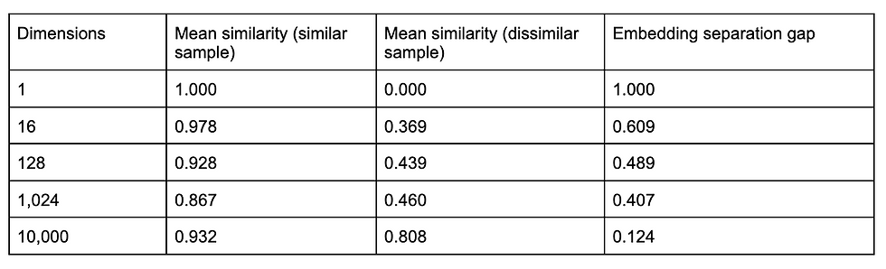
Embedding separation gap is calculated as mean similarity score for visually similar pairs minus mean similarity score for visually dissimilar pairs. Higher values indicate stronger apparent separation between the two hand-labelled groups.

The KDE plots below show the same pattern visually. At lower dimensions, the two groups form more clearly separated distributions. At 10,000 dimensions, the distance between the two groups is smaller.

Kdeplots:

1 dimension

n/a

16 dimensions

128 dimensions

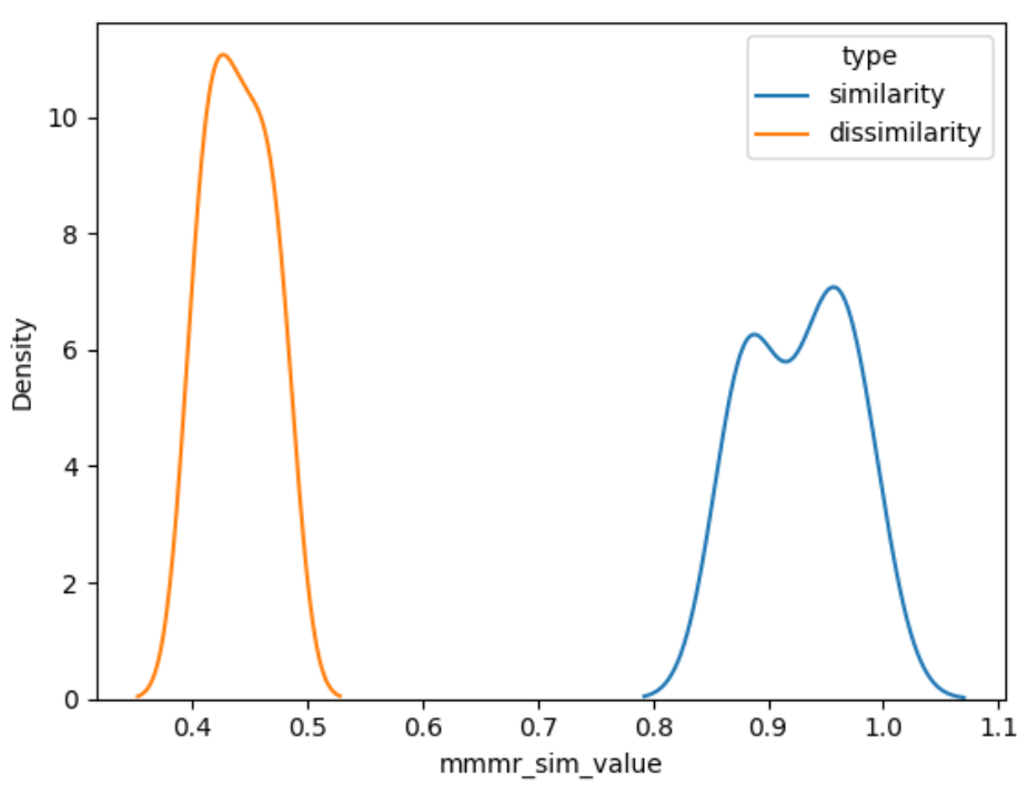
1,024 dimensions

10,000 dimensions

The decrease in distance between these different groups can be seen directly by plotting the Mean Separation of Similarity values as the number of dimensions varies.

The difference between mean similarity values is referred to as the Embedding separation gap. A clear non-linear pattern can be observed as the number of dimensions varies.

Discussion

Since the recent boom in AI, driven by large language models (LLMs), there's been an increased focus on the use of things like feature vectors or embeddings. This probably peaked with the widespread adoption of vector databases being used to carry out retrieval-augmented generation, otherwise known as RAG. 

Now, researchers and practitioners will be aware that not all embedding models are the same. Typically, embedding models tend to function as a universe, and the universe is the total range of input and training data that was used within the context of how an embedding model was created. In the case of LLMs, it will relate largely to the distribution of the training data that LLMs saw, and in other cases it will relate to the training data that that embedding model used. In the case of visual language models, for example, it will encompass both the images as well as the words or tokens that were used in the training of a model or training of that embedding model. 

When it comes to geospatial AI in particular, the idea of vectors and feature vectors is not new. This is primarily because remote sensing or Earth observation data, when used and extracted from satellites for scientific purposes, typically takes into account not just the visible RGB values of a place but also additional satellite band values, such as near-infrared (NIR) and other satellite bands. As such, it's not out of place for earth observation researchers and analysts to be aware of the need to account for this multidimensionality when doing their analysis or research. Typically, this is done using techniques such as Principal Component Analysis (PCA), which is to reduce the number of dimensions of the original data whilst preserving the underlying structure as much as possible. 

As the idea of scale as a solution to improved performance grew in Natural Language Processing (NLP) through the development of LLMs, a similar trend has been occurring in the space of Earth Observation (EO) or geospatial AI (GeoAI). GeoAI Large foundation models are being trained such that they can provide the same utility as LLMs do in NLP. However, unlike LLMs from NLP, GeoAI foundation models in EO tend to not be as explainable and their utility is not immediately obvious to practitioners. In some cases, these models are designed to function as representations of different locations such that other researchers can use this information once without having to replicate and reproduce that information themselves. There are a number of research projects going on aimed at developing these sorts of geospatial foundation models. However, as is likely to be the case, these models will largely reflect their training data as well as the universe that they considered as part of their development, just as is the case for LLMs. Taking, for example, two well-known embedding models: Google's Alpha Earth Foundation embeddings as well as LGND API's embedding models both are trained on large-scale EO data sets, not just cross-sectional but also temporal and multi-spectral. This means that these are able to generate embeddings that function as rich representations of different locations. In the case of Google Alpha Earth Foundations, these are available in 64 dimensions at the pixel level. In the case of LGND, they are derived from publicly available satellite data, such as those from Sentinel-2 and other similar missions, and have been reduced to 256 dimensions. 

Any use of dimension reduction techniques is associated with a loss of the underlying variation between observations in the data prior to that transformation. Namely, although there are benefits to reducing data size, there is also a penalty to be paid associated with loss of information, as well as potentially counterintuitive conclusions. Take, for example, the sample of positive and negative location pairs that we have looked at. When represented in their richest form (approximately 10,000 dimensions), we observe that the distance between the average cosine similarities of the similar and the dissimilar location pair samples is actually much closer than it appears once the dimensions are reduced. In fact, as the dimensions are reduced, we observe this bifurcation only increases. Perhaps this outcome can be seen as desirable, as it corresponds with what people perhaps intuitively feel when we say something is similar or something is dissimilar. However, in reality, it is a reductive form of representation and potentially exaggerates the difference between location pairs rather than allowing for more nuanced variations. Consider, for example, if we were to add an even more extremely dissimilar location pair and reduce the number of dimensions. We would not be able to say these two location pairs are any more dissimilar than the existing pairs that we found at one dimension, because effectively at that point everything is binary.

Unfortunately, it is not just the number of dimensions associated with an embedding model that may lead to unexpected outcomes. As has been alluded to, the nature of the training data, or rather the diversity of the training data used to create an embedding model, also shapes how good it is at differentiating between different feature vectors within that space. A model naively trained on a global and extremely heterogeneous set of data will be able to learn large differentiations and variations between all of those different locations. However, this may come at the cost of ignoring minor variations between feature vectors representing a dense Central Business District (CBD) and an inner city residential neighborhood, for example. This learning of broader patterns is likely going to be the result of the inherent skewed distribution of location data. Most locations in the world are natural places like fields, while urban and built-up locations are atypical and represent only a small proportion of the earth’s land surface. This skewed distribution means that any model trained naively on all locations is likely to learn the patterns associated with the majority classes whilst ignoring, to some degree, patterns associated with the minority classes. On the other hand, a model trained on a much narrower set of data, such as those only corresponding to human-inhabited locations, may do better at this sort of distinction. However, it too would fail at functioning effectively on out-of-distribution data, such as those associated with non-habitat human-habitated environments, such as the Arctic or the ocean. This is the challenge of using globalised embedding models. Initially, the allure of accounting for all of the world’s variation is appealing, however, in practice, it leads to only a small navigable space of useful distinctions. That small space is unfortunately not focused on urban locations when using a globally heterogeneous embedding model. 

In addition to the lossy nature of dimension reduction, we hope we have been able to demonstrate that using embedding models is not a bad thing and is often a significantly more efficient way of formalising fuzzy concepts such as similarity or dissimilarity. There are, however, no uses of embedding models without trade-offs, whether those trade-offs be explicit or implicit. It is our view that, where doing these forms of representation, the onus should be on the provider of the embedding models to be able to allow end users to customise or emphasise the characteristics that they deem to be appropriate, as opposed to a take-what-you-get model.

Conclusion

There is value and utility in using embedding models in the geospatial AI realm. Particularly, when moving towards an idea of accounting for a greater, richer representation of a place beyond just the RGB or pixel-level representations of a location. This does not mean simply using multi-spectral data sets and their associated embeddings, which has historically been the industry norm. This is because such embeddings are, by their very nature, opaque. For scientific purposes, where the embeddings function as a means of training models or carrying out regression and classification tasks, perhaps this is sufficient. However, industry use of such systems is unlikely to be successful without some form of steerability or explainability.

Use of techniques such as dimension reduction make it practical and tractable to work with embeddings by amelioring the need large compute, memory and storage and time requirements. However, the process of dimension reduction of a feature vector can change its relative positioning in the new embedding space and exaggerate its similarity or difference to other feature vectors. This means that if a multi-spectral data set or embedding model is then reduced in order to be used in a vector database, it is unlikely that the same behaviour occurring in that vector database corresponds to the original data and its original similarity or dissimilarity.

This work demonstrates that as the number of dimensions is reduced, the “embedding separation gap” (the difference between the mean similarity values of similar and dissimilar location pairs) increases. The effect of this is that applications making use of lower-dimensional embeddings are unlikely to be able to replicate their findings and results when using higher-dimensional representations of those same locations. That is to say, the conclusions are dependent on the number of dimensions of the data and not necessarily due to the underlying locations themselves.